banner


How To Draw A Figure In Latex

Table of Contents

How to depict diagrams in LaTeX with TikZ

Nice looking diagrams tin can be drawn in LaTeX with the versatile TikZ packet. This folio shows some examples that are useful for our CMS group.

TikZ should work out-of-the-box with \usepackage{tikz}, but the syntax is not so straightforward at first. To get started, accept a wait at these materials:

  • TeXample: A large database of unproblematic and advanced examples with a physics department, including a Feynman diagram and a Standard Model diagram. This website will be superseded past TikZ.net.

  • For Feynman diagrams, please encounter this page.

Command regions

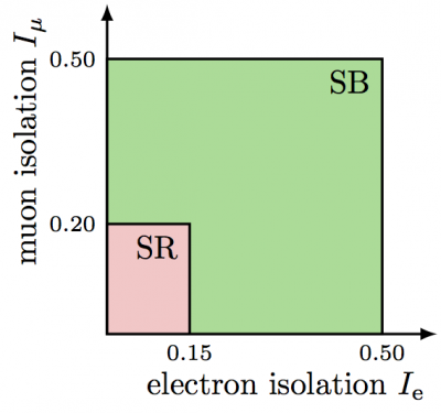
Control regions are simple enough to draw in TikZ, since it is in 2d and only requires to draw arrows, rectangulars and nodes (nodes are unproblematic points, which useful for labeling). Below are 2 examples. The tex file containing both tin can be constitute here.

A simple instance of 2D axes and colored rectangles, with custom colors defined in the preamble:

            \            definecolor            {            mylightred}{RGB}{255,​200,​200}              \              definecolor              {mylightblue}{RGB}{172,​188,​63}              \              definecolor{mylightgreen}{RGB}{150,​220,​150            }          
                \begin                {                                  tikzpicture                                }[                calibration=half dozen                ]                % ascertain to modify easily                                \                def                \isoe                {                0.15}                  \                  def                  \isomu                  {0.20}                  \                  def                  \isoSB                  {0.50}                  \                  def                  \isomax{0.60                }                % axes                \draw                [                ->,thick                ]                (0,0) -- (0,\isomax)   node[                at cease,left=24pt,rotate=90                ]                {                muon isolation                  $I_\mu$                  };                  \draw                  [                  ->,thick                  ]                  (0,0) -- (\isomax,0)   node[                  at end,below=16pt,left                  ]                  {electron isolation                  $I_\text{eastward}$                                };                % boxes                \draw                [                thick,fill=mylightgreen                ]                (0,0) rectangle (\isoSB,\isoSB)   node[                anchor=northward eastward                ]                {                SB};                  \draw                  [                  thick,fill up=mylightred                  ]                  (0,0) rectangle (\isoe,\isomu)   node[                  anchor=northward due east] {SR                };                % labels                \describe                (0,\isomu) node[                anchor=due east                ]                {                                  \scriptsize                  $\isomu$                  }                  (0,\isoSB) node[                  anchor=east                  ]                  {                  \scriptsize                  $\isoSB$                  }                  (\isoe, 0) node[                  anchor=n                  ]                  {                  \scriptsize                  $\isoe$                  }                  (\isoSB,0) node[                  ballast=n                  ]                  {                  \scriptsize                  $\isoSB$                  };                  \end                  {                  tikzpicture                                }              

A simple case of a rectangle, dashed lines and using the scope environment to modify the coordinate system locally in the lawmaking. In this example the coordinate system is shifted and scaled, but information technology also possible to do rotations (rotate=60) or scale only horizontally (vertically) with xscale=1.5 (yscale=1.5).

                \begin                {                                  tikzpicture                                }[                scale=four                ]                % axes                \draw                [                thick                ]                (0,0) rectangle (one,ane);                % boxes                \draw                [                dashed,thick                ]                (0.5,-0.1) -- (0.5,1);                \draw                [                dashed,thick                ]                (-0.1,0.5) -- (1,0.v);                % labels                \draw                (0,0.75) node[                anchor=due east                ]                {                Bone}                  (0,0.25) node[                  anchor=due east                  ]                  {SS}                  (0.25,0) node[                  ballast=north                  ]                  {SR}                  (0.75,0) node[                  ballast=northward                  ]                  {SB};                  \describe                  (0.25,0.75) node                  {QCD}                  (0.75,0.25) node[                  text width=xl,align=middle                  ]                  {QCD\                  \shape                                };                % arrows                \begin                {                                  scope                  }[                  shift={(0.51,0.52)},scale=0.3                  ]                  \describe                  [                  ->,thick                  ]                  (0.5,-0.five) -- (-0.5,0.5)     node[                  midway, above=6pt, right=1pt                  ]                  {                  \scriptsize                  $F$                  };                  \end                  {                  scope                  }                  \end                  {                  tikzpicture                                }              

Sets

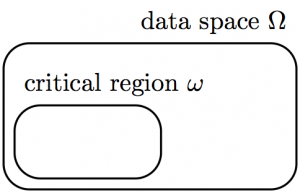
Another simple example of a rectangle with rounded corners:

sets.tex
                    \                    documentclass                    {                    commodity}                      \                      usepackage{tikz                    }                    % split figures into pages                    \                    usepackage                    [                    active,tightpage                    ]{                    preview}                      \PreviewEnvironment                      {tikzpicture}                      \                      setlength                      \PreviewBorder{1pt                    }                    %                    \begin                    {                                          document                                        }                    % SET: critical region                    \begin                    {                                          tikzpicture                      }[                      calibration=ane.0                      ]                      \draw                      [                      black,rounded corners=ten,thick                      ]                      (0,0) rectangle (four,2)      node[                      above left                      ]                      {data space                      $\Omega$                      };                      \draw                      [                      black,rounded corners=10,thick,shift={(0.15,0.xv)}                      ]                      (ii,0) rectangle (0,one)      node[                      above right                      ]                      {critical region                      $\omega$                      };                      \cease                      {                      tikzpicture                      }                      \end                      {                      document                                        }                  

Flowchart

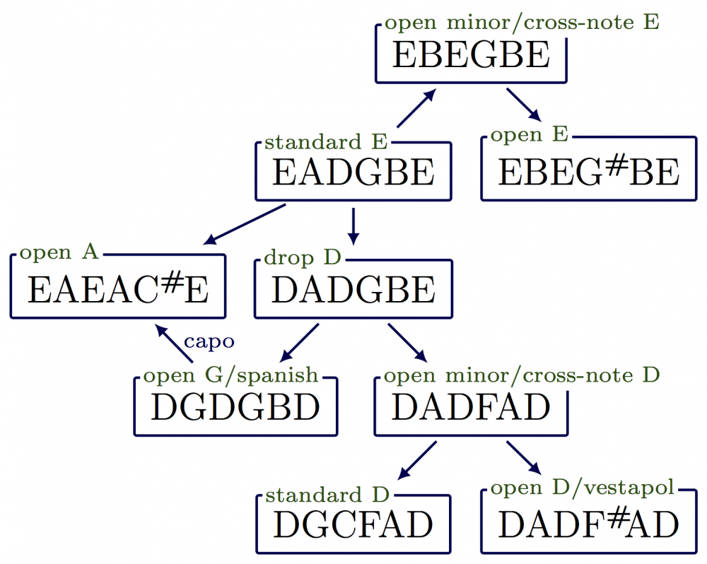
Example of a flow chart past using predefined drawing styles and a predefined box with \def and arguments (full lawmaking):

                \begin                {                                  tikzpicture                  }[                  xscale=1.iii,yscale=one.ii,                     fscale/.style={font=\relsize{#1}},                     arrow/.mode={->,thick,mydarkblue,shorten <=2,shorten >=iv},                     sarrow/.style={->,thick,mydarkblue,shorten <=2,shorten >=6}                  ]                  \                  def                  \c                  {0.7}                  \                  def                  \m                  {v}                  \                  def                  \tuning(#1,#2,#3,#4,#5){                  \node                  [                  draw=mydarkblue,thick,rounded corners=\c,inner sep=\1000                                    ]                  (#one) at (#2,#3)                  [                  fscale=i.2,ballast=south                  ]                  {#4};                  \node                  [                  make full=white,inner sep=i                  ]                  at (#1.due north west)                  [                  fscale=-2,right=ii,ballast=w,text=mydarkgreen                  ]                  {#5};                                }                % TUNINGS                \tuning(E,  1, 5, EBEGBE,      open minor/cross-note E)                \tuning(D,  0, iv, EADGBE,      standard E)                \tuning(Dr, ii, 4, EBEG\sh                \,Be, open E)                \tuning(C,  0, 3, DADGBE,      driblet D)                \tuning(Cl,-2, 3, EAEAC\sh                \,East, open up A)                \tuning(Bl,-1, two, DGDGBD,      open G/spanish)                \tuning(Br, i, two, DADFAD,      open small/cross-note D)                \tuning(A,  0, 1, DGCFAD,      standard D)                \tuning(Ar, ii, 1, DADF\sh                Ad,  open up D/vestapol)                % Pointer                \depict                [                sarrow,<-                ]                (E)  -- (D);                \draw                [                sarrow                ]                (Eastward)  -- (Dr);                \draw                [                arrow                ]                (D)  -- (C);                \draw                [                sarrow                ]                (D)  -- (Cl);                \draw                [                sarrow,<-                ]                (Cl) -- (Bl) node[                fscale=-ii,midway,in a higher place=one,right=-2                ]                {                capo};                  \draw                  [                  sarrow                  ]                  (C)  -- (Bl);                  \draw                  [                  sarrow                  ]                  (C)  -- (Br);                  \draw                  [                  sarrow                  ]                  (Br) -- (A);                  \draw                  [                  sarrow                  ]                  (Br) -- (Ar);                  \terminate                  {                  tikzpicture                                }              

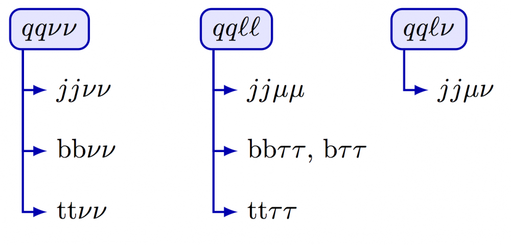
Example of a node with arrows to text below it (full code). Annotation the use of |- between coordinates to draw a line that beginning goes downwardly vertically and and so horizontally. Vice versa can be done with -|. The \strut control is used to ensure that the text line has a stock-still superlative.

                \brainstorm                {                                  tikzpicture                                }[                yscale=0.8,anchor=w                ]                % Beginning Cavalcade                \node                [                anchor=west,draw=myblue,fill=mylightblue,thick,rounded corners=4,inner sep=1.5pt                ]                (L) at (0,four)                {                                  \;\strut                                    $qq\nu                    \nu$                  \;};                  \node                  (L1) at (0.five,iii)                  {                  \strut                  $jj\nu                    \nu$                  };                  \node                  (L2) at (0.5,2)                  {                  \strut                  bb$\nu                    \nu$                  };                  \node                  (L3) at (0.5,1)                  {                  \strut                  tt$\nu                    \nu$                                };                \describe                [                ->,myblue,thick                ]                (Fifty.south w)++(0.18,0) |- (L1.west);                \draw                [                ->,myblue,thick                ]                (50.s west)++(0.eighteen,0) |- (L2.west);                \draw                [                ->,myblue,thick                ]                (L.south westward)++(0.18,0) |- (L3.west);                % SECOND COLUMN                \begin                {                                  scope                  }[                  shift={(ii.5,0)}                  ]                  \node                  [                  depict=myblue,fill=mylightblue,thick,rounded corners=4,inner sep=1.5pt                  ]                  (Yard) at (0,4)                  {\;\strut                  $qq\ell                    \ell$                  \;};                  \node                  (M1) at (0.5,3)                  {                  \strut                  $jj\mu                    \mu$                  };                  \node                  (M2) at (0.5,2)                  {                  \strut                  bb$\tau                    \tau$, b$\tau                    \tau$                  };                  \node                  (M3) at (0.v,one)                  {                  \strut                  tt$\tau                    \tau$                  };                  \draw                  [                  ->,myblue,thick                  ]                  (M.south w)++(0.18,0) |- (M1.w);                  \draw                  [                  ->,myblue,thick                  ]                  (Thou.south west)++(0.xviii,0) |- (M2.westward);                  \describe                  [                  ->,myblue,thick                  ]                  (M.south w)++(0.18,0) |- (M3.west);                  \end                  {                  scope                                }                % Tertiary COLUMN                \begin                {                                  scope                  }[                  shift={(v.0,0)}                  ]                  \node                  [                  draw=myblue,make full=mylightblue,thick,rounded corners=4,inner sep=one.5pt                  ]                  (R) at (0,four)                  {\;\strut                  $qq\ell                    \nu$                  \;};                  \node                  (R1) at (0.5,3)                  {                  \strut                  $jj\mu                    \nu$                  };                  \describe                  [                  ->,myblue,thick                  ]                  (R.south west)++(0.18,0) |- (R1.west);                  \end                  {                  scope                  }                  \stop                  {                  tikzpicture                                }              

Cantlet models

Hither are some case of making dots and circles, again with predefined colors in the preamle (see consummate code for all three figures):

            % colors            \            definecolor            {            mylightred}{RGB}{255,210,210}              \              definecolor              {mydarkred}{RGB}{140,40,40}              \              definecolor{mydarkblue}{RGB}{l,70,190            }          

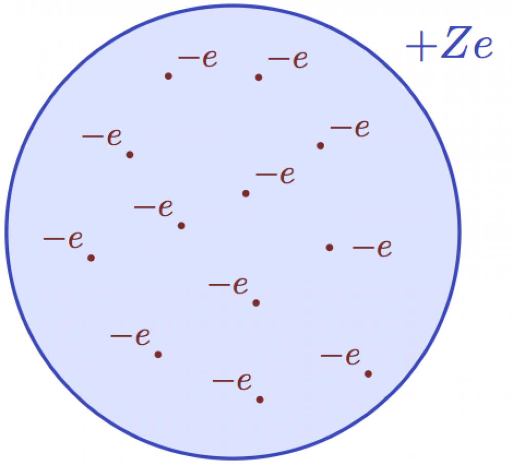
Thomson model: uniformly and positively charged sphere with negatively charged electrons.

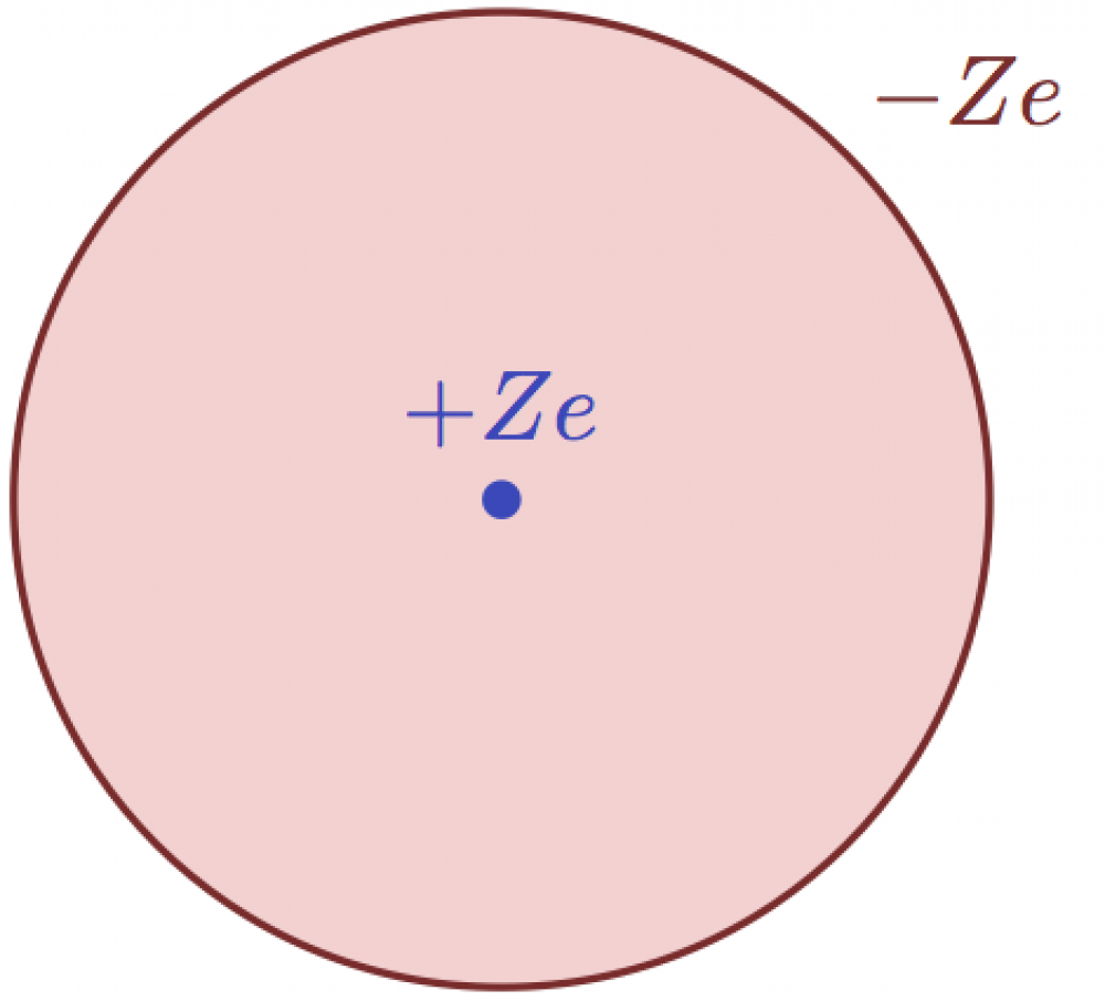
Simplified Rutherford model: positively charged nucleus, uniformly and negatively charged sphere.

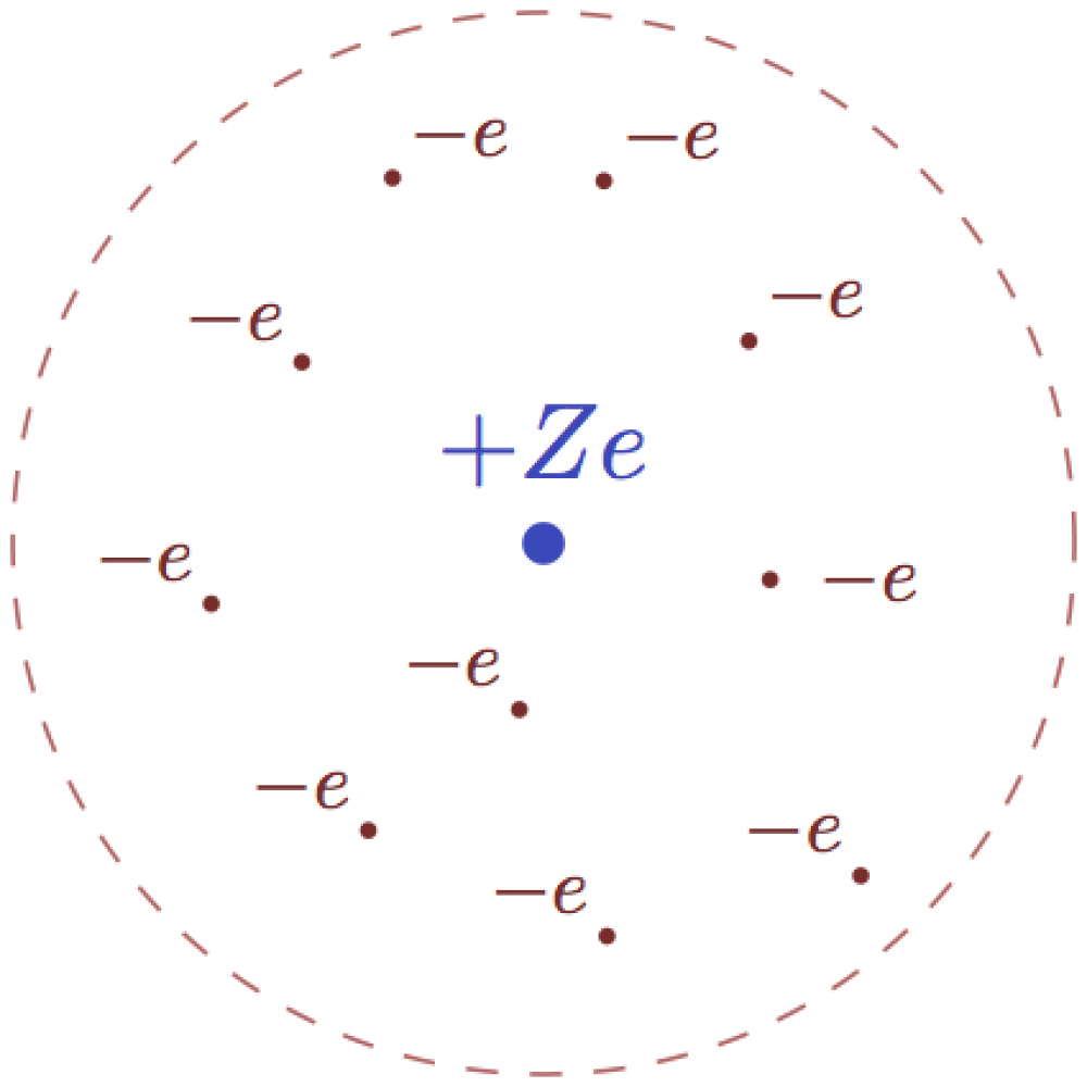
Rutherford model: positively charged nucleus, with negatively charged "corpuscles" (electrons).

            % Cantlet MODEL: Simplified Rutherford model            \begin            {                          tikzpicture              }[              scale=ane              ]              \coordinate              (O)  at (0,0);              \draw              [              mylightred,fill up              ]              (O) circle (50pt);              \depict              [              mydarkred,thick              ]              (O) circle (50pt) node[              in a higher place right=34pt              ]              {              $-Ze$              };              \fill              [              radius=ii.0pt,mydarkblue              ]              (O) circle node[              in a higher place=2pt              ]              {              $+Ze$              };              \end              {              tikzpicture                        }          

Vector sums & projections

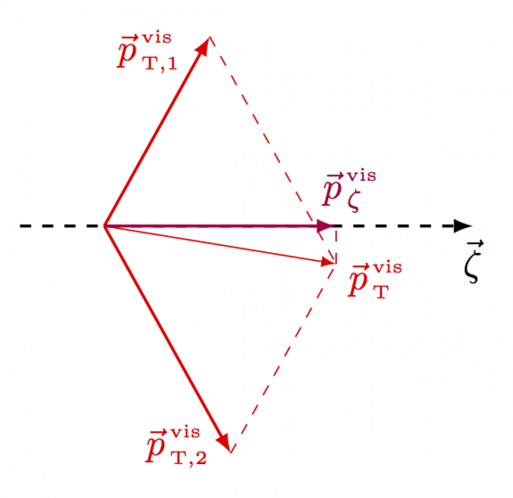
Here is a simple instance of projecting vectors, inspired by Jang (2006) [Fig. iii.five]. The tex file tin can be found here.

By using \coordinate, your code become more readable, and more like shooting fish in a barrel to adapt with new coordinate values.

            \coordinate            (A) at (1,2);            \coordinate            (B) at (2,-three);            \draw            (A) -- (B);

In addition, you tin use the TikZ library calc to practice arithmetic with the coordinates, e.one thousand.

            \coordinate            (AB) at ($(A)+(B)$);            % (3,-i)          

And yous tin can besides acces the 10 and y components with let \p. E.g. to ascertain coordinate P every bit a projection of A onto the x-axis:

            \coordinate            (A)  at (1,ii);            \path            let            \p            {            A}=(A) in coordinate (P) at (\ten{A            },0);            % (1,0), projection of A          
                \usetikzlibrary                {                calc                }                % to sum coordinates                \begin                {                                  tikzpicture                                }                % vector labels                \                def                \pT                {                                  \vv                  {p}^\text                  {                  \tiny                  \,vis}_\text                  {                  \tiny                  \,T}}                  \                  def                  \pTA                  {                  \vv                  {p}^\text                  {                  \tiny                  \,vis}_\text                  {                  \tiny                  \,T,i}}                  \                  def                  \pTB                  {                  \vv                  {p}^\text                  {                  \tiny                  \,vis}_\text                  {                  \tiny\,T,2}                }                % define bespeak                \coordinate                (O)  at (0.0, 0.0);                \coordinate                (Z)  at (3.5, 0.0);                \coordinate                (A)  at (ane.0, 1.eight);                \coordinate                (B)  at (1.2,-2.xvi);                \coordinate                (AB) at ($(A)+(B)$);                \path                let                \p                {                AB}=(AB) in coordinate (P) at (\10{AB                },0);                % projection                % axis                \draw                [                ->,thick,dashed                ]                (-0.8,0) -- (Z)     node[                at end,beneath                ]                {                                  $\vv                    {                    \zeta}$                                };                % main vectors                \draw                [                ->,thick,colour=red                ]                (O) -- (A)     node[                beneath=4pt,left=4pt,color=red                ]                {                                  $\pTA$                  };                  \draw                  [                  ->,thick,color=cherry                  ]                  (O) -- (B)     node[                  above=2pt,left=2pt,color=red                  ]                  {                  $\pTB$                  };                  \draw                  [                  ->,color=scarlet                  ]                  (O) -- (AB)     node[                  below=4pt,correct,color=red,scale=1                  ]                  {                  $\pT$                                };                %{$\sq\pTA+\,\pTB$};                % helplines                \depict                [                dashed,colour=red                ]                (A) -- (AB);                \draw                [                dashed,color=crimson                ]                (B) -- (AB);                \draw                [                dashed,colour=royal                ]                (AB) -- (P);                % vector sum                \draw                [                ->,thick,color=purple                ]                (O) -- (P)     node[                right=4pt,above,color=imperial                ]                {                                  $\vv                    {p}^\text                    {                    \tiny                    \,vis}_{                    \tiny                    \,\zeta}$                  };                  \end                  {                  tikzpicture                                }              

with the predefined command

            \            newcommand*{                          \vv              }[              ane              ]{              \vec              {              \mkern0mu#1}            }          

in the preamble for ameliorate alignment of the vector arrow \vec over math symbols.

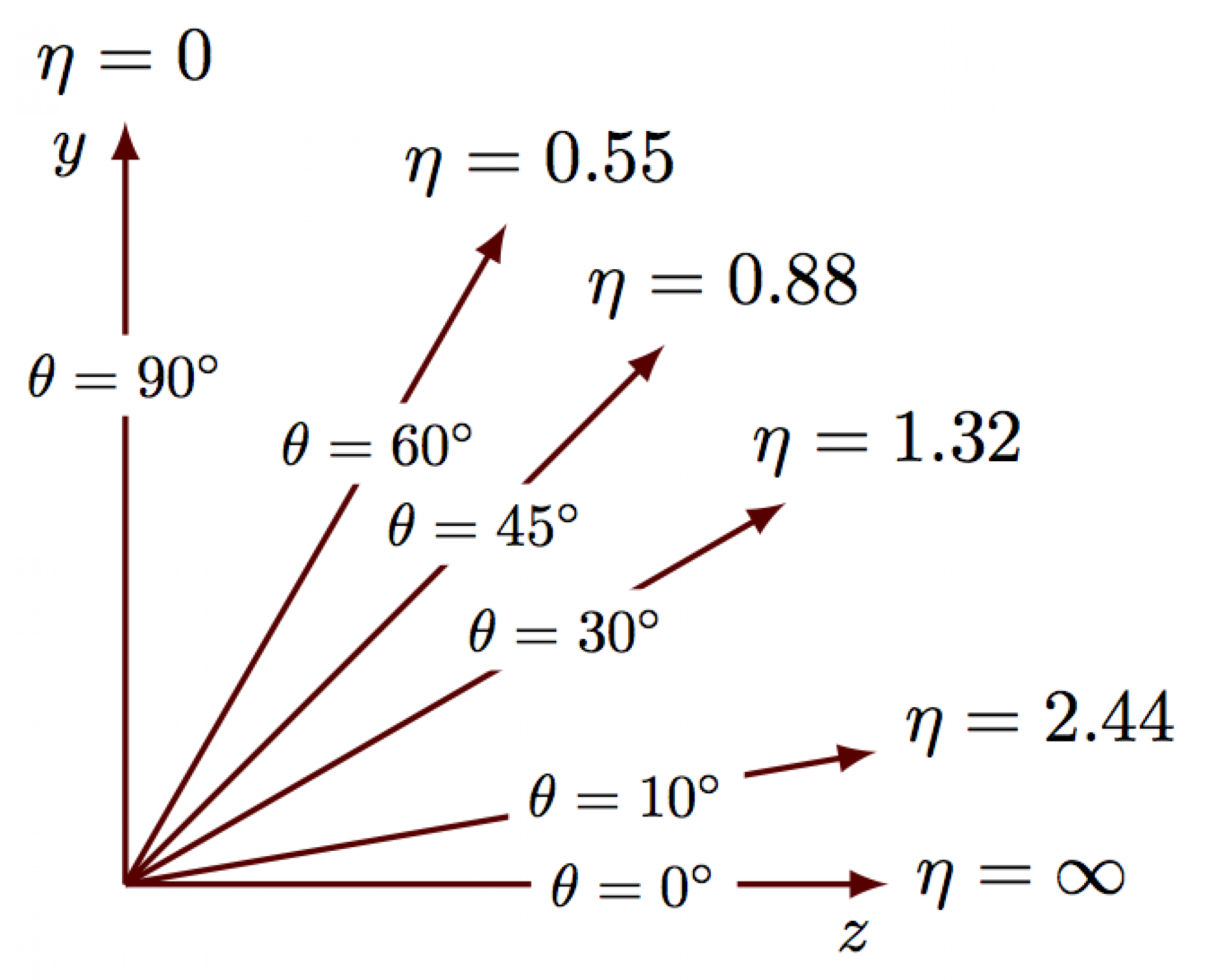
For-loops: Pseudorapidity 𝜂 and polar angle 𝜃

Hither are two example of using a for-loop with TikZ's \foreach. In this example nosotros loop over two variables. Full code tin be constitute hither.

                \begin                {                                  tikzpicture                                }[                calibration=3                ]                % limits                \                def                \R                {                one.ii                }                % axis labels                \node                [                below=5pt,left=2pt                ]                at (0,\R)                {                                  $y$                  };                  \node                  [                  left=5pt,below=2pt                  ]                  at (\R,0)                  {                  $z$                                };                % lines                \foreach                \t                in                {                90,60,45,30,ten,0}{                  \draw                  [                  ->,black!60!scarlet,thick                  ]                  (0,0) -- ({                  \R*cos(\t)},{                  \R*sin(\t)})       node[                  anchor=180+\t,black                  ]                  {                  $\theta=\t$                  };                  }                  \end                  {                  tikzpicture                                }              


                \brainstorm                {                                  tikzpicture                                }[                calibration=3                ]                % limits                \                def                \R                {                1.two                }                % axis labels                \node                [                scale=0.nine,below=5pt,left=2pt                ]                at (0,\R)                {                                  $y$                  };                  \node                  [                  scale=0.9,left=5pt,beneath=2pt                  ]                  at (\R,0)                  {                  $z$                                };                % lines                \foreach                \t/\e                in                {                ninety/0,60/0.55,45/0.88,30/ane.32,10/2.44,0/\infty                  }{                  \draw                  [                  ->,black!threescore!red,thick                  ]                  (0,0) -- ({                  \R*cos(\t)},{                  \R*sin(\t)})       node[                  anchor=180+\t,blackness                  ]                  {                  $\eta=\e$                  };                  \node                  [                  fill=white,scale=0.8                  ]                  at ({0.eight*cos(\t)},{0.8*sin(\t)})                  {                  $\theta=\t^\circ$                  };                  }                  \stop                  {                  tikzpicture                                }              
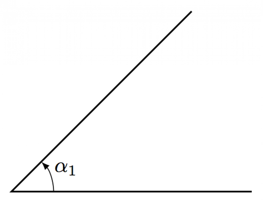


Labeling angles

Here are 2 different ways of labeling an angle: using \draw pic or \pic. Both requite the same result and need the TikZ libraries angles and quotes.

                \usetikzlibrary                {                angles,quotes                }                % for pic (angle labels)                \begin                {                                  tikzpicture                                }                % define point                \coordinate                (A)  at (3, 3);                \coordinate                (O)  at (0, 0);                \coordinate                (B)  at (4, 0);                % angle                                \describe                [                thick                ]                (A) -- (O) -- (B);                \draw                movie[                ->,"$\alpha_1$",draw=blackness,angle radius=20,bending eccentricity=1.4                ]                {                bending = B--O--A                };                %\movie [describe,"$\alpha_1$",angle radius=20,->,bending eccentricity=1.4]                %  {angle = B--O--A};                \end                {                                  tikzpicture                                }              

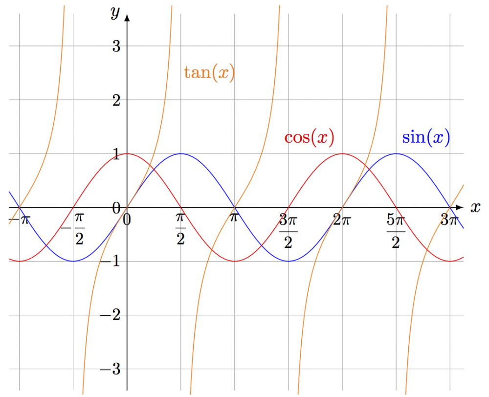
Plotting second functions

Examples of plotting trigonometric functions with two unlike methods. Total code (borrowed from a friend) can exist plant hither.

With \draw plot(\10,{f(\x r)}) (including \usepackage{tikz} for \dfrac):

                \begin                {                                  tikzpicture                                }[                domain=-pi:pi,xscale=2/pi                ]                % limits                \                def                \xa                {                                  -pi-0.three}                  \                  def                  \xb                  {3*pi+0.4}                  \                  def                  \ya                  {-three.4}                  \                  def                  \yb                  {                  3.6}                  \                  def                  \N{100                }                % number of points                % axes & filigree                \draw                [                xstep=pi/2,very thin, color=grey                ]                (\xa,\ya) grid (\xb,\yb);                \depict                [                ->                ]                (\xa,0) -- (\xb,0)     node[                right                ]                {                                  $ten$                  };                  \draw                  [                  ->                  ]                  (0,\ya) -- (0,\yb)     node[                  left                  ]                  {                  $y$                                };                % ticks                \depict                [                ]                % x                node[                below,calibration=0.nine                ]                at ( -pi,   0)                {                                  $-\pi$                  }                  node[                  below,scale=0.9                  ]                  at ( -pi/two, 0)                  {                  $-\dfrac                    {                    \pi}{2}$                  }                  node[                  beneath,calibration=0.9                  ]                  at (  pi,   0)                  {                  $\pi$                  }                  node[                  below,scale=0.9                  ]                  at (     0, 0)                  {0}                  node[                  below,scale=0.9                  ]                  at (  pi/two, 0)                  {                  $\dfrac                    {                    \pi}{2}$                  }                  node[                  beneath,scale=0.9                  ]                  at (  pi,   0)                  {                  $\pi$                  }                  node[                  beneath,calibration=0.ix                  ]                  at (3*pi/2, 0)                  {                  $\dfrac                    {three\pi}{2}$                  }                  node[                  below,scale=0.9                  ]                  at (two*pi,   0)                  {                  $2\pi$                  }                  node[                  below,scale=0.nine                  ]                  at (5*pi/2, 0)                  {                  $\dfrac                    {5\pi}{2}$                  }                  node[                  below,scale=0.9                  ]                  at (three*pi,   0)                  {                  $3\pi$                                };                \draw                [                ]                % y                node[                left,scale=0.ix                ]                at ( 0,  3)                {                                  $3$                  }                  node[                  left,scale=0.ix                  ]                  at ( 0,  two)                  {                  $2$                  }                  node[                  left,scale=0.9                  ]                  at ( 0,  1)                  {                  $one$                  }                  node[                  left,scale=0.9                  ]                  at ( 0,  0)                  {                  $0$                  }                  node[                  left,calibration=0.ix                  ]                  at ( 0, -ane)                  {                  $-1$                  }                  node[                  left,scale=0.ix                  ]                  at ( 0, -2)                  {                  $-2$                  }                  node[                  left,scale=0.nine                  ]                  at ( 0, -3)                  {                  $-3$                                };                % office                \                def                \ea                {                0.28}                  \                  def                  \eb{0.26                }                \draw                [                colour=blue,samples=\Northward,domain=\xa:\xb                                ]                % SIN                plot(\ten,{                sin(\x                  r)                })                % r for radians                node[                above correct                ]                at (5*pi/2,1)                {                                  $\sin(x)$                                };                \draw                [                color=red,samples=\Northward,domain=\xa:\xb                                ]                % COS                plot(\x,{                cos(\x                  r)})     node[                  in a higher place left                  ]                  at (2*pi,1)                  {                  $\cos(10)$                                };                \draw                [                color=orangish                ]                % TAN                plot[                samples=\N,domain=                  \xa                  :   -pi/2-\eb                                ]                (\x,                {                tan(\x                  r)})     plot[                  samples=\N,domain=  -pi/2+\ea:   pi/2-\eb                                    ]                  (\x,                  {tan(\x                  r)})     plot[                  samples=\North,domain=   pi/two+\ea: 3*pi/2-\eb                                    ]                  (\x,                  {tan(\x                  r)})     plot[                  samples=\N,domain= 3*pi/2+\ea: 5*pi/two-\eb                                    ]                  (\x,                  {tan(\x                  r)})     plot[                  samples=\N,domain= 5*pi/two+\ea:                    \xb                                    ]                  (\x,                  {tan(\ten                  r)})     node[                  samples=\N,correct=-2pt                  ]                  at (pi/2,two.v)                  {                  $\tan(x)$                  };                  \terminate                  {                  tikzpicture                                }              

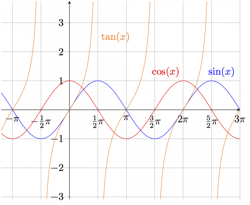
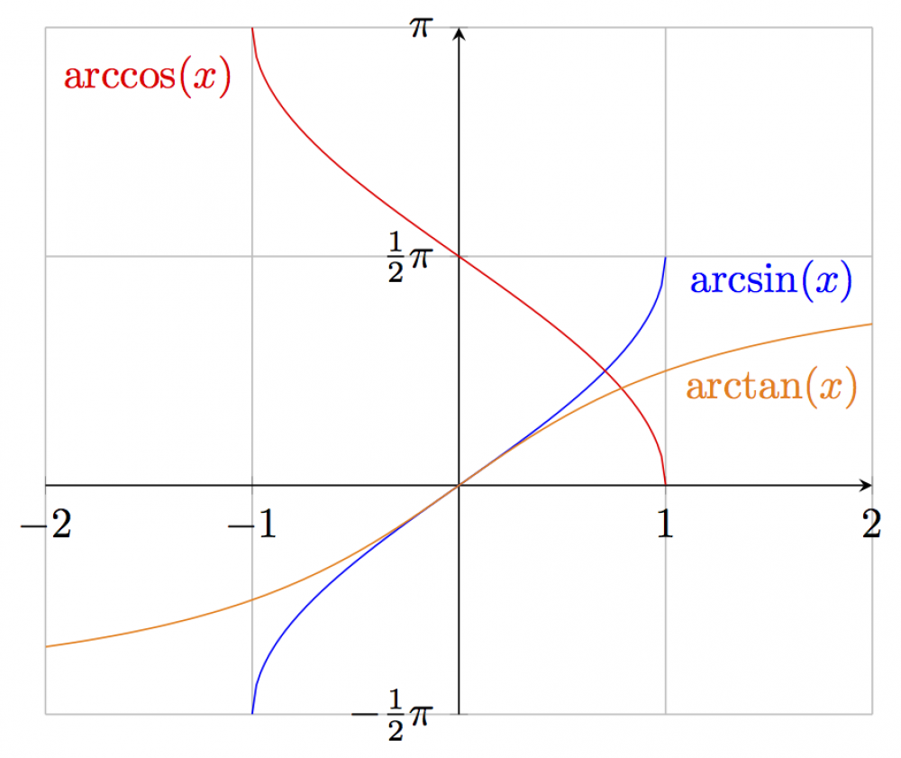
With \addplot in the centrality environment.

                \brainstorm                {                                  tikzpicture                  }[                  scale=1.2                  ]                  \begin                  {                  axis                  }[enlargelimits=false,              axis lines=middle,              scale=1.2,              xtick={-3.15159, -1.57080, 0,                      one.57080,  3.15159, four.71239,                      6.28318,  7.85398, 9.42478                  },               xticklabels={                  $-\pi$,                  $-\frac                    {1}{2}                    \pi$, 0,                  $\frac                    {1}{2}                    \pi$,                  $\pi$,                  $\frac                    {three}{2}                    \pi$,                  $2\pi$,                  $\frac                    {5}{2}                    \pi$,                  $3\pi$                  },              ytick={-iii,-2,-ane,0,1,2,iii                },              filigree=major,                % only a grid on the defined ticks                samples=100                % number of points                ]                % sin                \addplot                [                blue,no marks,domain=-1.2*pi:iii*pi                ]{                sin(deg(10))                };                % deg to convert radians                \node                [                right=10pt,above                ]                at (centrality cs:5*pi/two,i){                \color                  {blue}                  $\sin(ten)$                                };                % cos                \addplot                [                ruby-red,no marks,domain=-ane.2*pi:3*pi                ]                {                cos(deg(x))};                  \node                  [                  above left                  ]                  at (axis cs:2*pi,1){\                  colour                  {red}                  $\cos(x)$                                };                % tan, multiple parts because of singularities                \addplot                [                orange,no marks,domain=-1.2*pi:-0.583*pi,                                ]{                tan(deg(x))};                  \addplot                  [                  orange,no marks,domain=-0.4*pi:5*pi/12,                                    ]{tan(deg(x))};                  \addplot                  [                  orangish,no marks,domain=27*pi/45:17*pi/12,                                    ]{tan(deg(x))};                  \addplot                  [                  orangish,no marks,domain=1.6*pi:29*pi/12,                                    ]{tan(deg(x))};                  \addplot                  [                  orangish,no marks,domain=2.6*pi:36*pi/12,                                    ]{tan(deg(x))};                  \node                  [                  right                  ]                  at (axis cs:pi/2,2.v){\                  color                  {orange}                  $\tan(10)$                  };                  \end                  {                  centrality                  }                  \end                  {                  tikzpicture                                }              

                \begin                {                                  tikzpicture                  }                  \begin                  {                  axis                  }[                  enlargelimits=false,              axis lines=middle,              xtick={-2,-i,0,one,2},              ytick={-1.570780, i.570780, 3.14159},              yticklabels={                    $-\frac                      {1}{2}                      \pi$,$\frac                      {one}{2}                      \pi$,$\pi$                  },              grid=major,              samples=100                                ]                % arcsin                \addplot                [                domain=-1:one,no marks,blue                ]                {                rad(asin(x))};                  \node                  at (axis cs:1.52,1.4){\                  color                  {bluish}                  $\arcsin(x)$                                };                % arccos                \addplot                [                domain=-1:one,no marks,red                ]                {                rad(acos(10))};                  \node                  at (axis cs:-1.v,2.8){\                  color                  {reddish}                  $\arccos(10)$                                };                % arctan                \addplot                [                domain=-ii:2,no marks,orange                ]                {                rad(atan(10))};                  \node                  at (axis cs:i.52,.67){\                  color                  {orange}                  $\arctan(x)$                  };                  \end                  {                  axis                  }                  \cease                  {                  tikzpicture                                }              
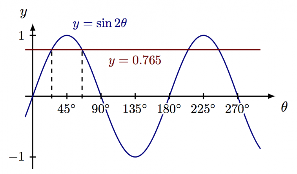
Total lawmaking:

                \brainstorm                {                                  tikzpicture                  }[                  scale=1.5,xscale=1/80                  ]                  \                  def                  \N                  {sixty}                  \                  def                  \xmin                  {-10}                  \                  def                  \xmax                  {320}                  \                  def                  \ymin                  {-1.2}                  \                  def                  \ymax                  {1.2}                  \                  def                  \tmin                  {-x}                  \                  def                  \tmax                  {300}                  \                  def                  \blue                  {black!50!bluish},                  \                  def                  \carmine                  {black!50!red}                  \                  def                  \value                  {0.765}                  \                  def                  \Dtheta{20                }                % axes                \draw                [                ->,thick                ]                (\xmin,0) -- (\xmax,0)     node[                anchor=north west                ]                {                                  $\theta$                  };                  \draw                  [                  ->,thick                  ]                  (0,\ymin) -- (0,\ymax)     node[                  anchor=south east                  ]                  {                  $y$                                };                % plots                \describe                [                thick,\blue,variable=\t,domain=\tmin:\tmax,samples=\N,smoothen                ]                plot (\t,{                sin(2*\t)                });                \draw                [                thick,\carmine,variable=\t,domain=\tmin:\tmax,samples=\North,smooth                ]                plot (\t,\value);                % office labels                \node                [                                  \blue,above correct=1pt,scale=0.9                ]                at (45,i)                {                                  $y=\sinii\theta$                  };                  \node                  [                                      \scarlet, below=1pt,scale=0.9                  ]                  at (135,\value)                  {                  $y=\value$                                };                % numerical solutions                \draw                [                dashed,thick                ]                (45-\Dtheta,-\value*0.05) -- (45-\Dtheta,\value*1.05);                \draw                [                dashed,thick                ]                (45+\Dtheta,-\value*0.05) -- (45+\Dtheta,\value*ane.05);                % ticks                \foreach                \x                in                {                45,90,135,180,225,270}{                  \draw                  [                  thick                  ]                  (\x,0.05) -- (\x,-0.05) node[                  below,scale=0.9                  ]                  {                  \contour                  {white}{                  $\x^\circ$                  }};}                  \foreach                  \y                  in                  {1,-1}{                  \draw                  [                  thick                  ]                  (4,\y) -- (-4,\y) node[                  left,scale=0.9                  ]                  {                  $\y$                  };}                  \cease                  {                  tikzpicture                                }              

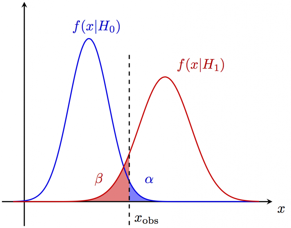
Here is an instance from statistics, using the pgfplots library fillbetween to make a shaded area between a function and a path. The total code tin be found here. The gauss role is defined as

            \pgfmathdeclarefunction            {            gauss}{3            }{            %            \pgfmathparse            {            i/(#3*sqrt(2*pi))*exp(-((#1-#2)^two)/(2*#3^ii))            }            %            }          
                % GAUSSIANs                \brainstorm                {                                  tikzpicture                  }                  \                  def                  \q                  {13.viii};                  \                  def                  \B                  {8.five};                  \                  def                  \S                  {xviii.5};                  \                  def                  \Bs                  {two.60};                  \                  def                  \Ss                  {iii.twoscore};                  \                  def                  \xmax                  {                  \Due south+3.two*\Ss                  };                  \                  def                  \ymin                  {{-0.15*gauss(\B,\B,\Bs)}};                  \begin                  {                  axis                  }[every axis plot post/.append manner={                  marking=none,domain={-0.05*(\xmax)}:{1.08*\xmax                  },samples=fourscore,smoothen},                xmin={-0.one*(\xmax)}, xmax=\xmax,                ymin=\ymin, ymax={1.i*gauss(\B,\B,\Bs)                },                centrality lines=middle,                axis line way=thick,                enlargelimits=upper,                % extend the axes a bit to the right and acme                ticks=none,                xlabel=$x$,                every axis x characterization/.mode={                at={(current axis.right of origin)},anchor=north westward                },                ]                % plots                \addplot                [                name path=B,thick,black!10!blue                ]                {                gauss(x,\B,\Bs)};                  \addplot                  [                  proper name path=S,thick,black!ten!red                                    ]                  {gauss(x,\S,\Ss)};                  \addplot                  [                  black,dashed,name path=Q,thick                  ]                  coordinates                  {(\q,                  {0.90*gauss(\B,\B,\Bs)}) (\q,                  \ymin)}                  node[                  beneath=2pt,ballast=southward west                  ]                  {                  $x_\text{obs}$                                };                % fill                \path                [                name path=xaxis                ]                (0,0) -- (\xmax,0);                \addplot                [                white!50!blue                ]                fill between[                of=xaxis and B, soft clip={domain=\q:\xmax}                  ];                  \addplot                  [                  white!50!blood-red                  ]                  fill up betwixt[                  of=xaxis and S, soft clip={domain=0:\q                  }                ];                % labels                \node                [                above,      black!20!bluish                ]                at (1.12*\B,{                gauss(\B,\B,\Bs)})                  {                                      $f(x|H_0)$                                    };                  \node                  [                  in a higher place right,black!20!red                                    ]                  at (one.05*\Southward,{gauss(\S,\S,\Ss)})                  {                                      $f(x|H_1)$                                    };                  \node                  [                  above left, black!20!red                                    ]                  at ({0.8*\q                  },{gauss(1.07*\q,\B,\Bs)})                  {                  \strut                  $\beta$                  };                  \node                  [                  above right,black!20!bluish                  ]                  at ({1.1*\q                  },{gauss(1.07*\q,\B,\Bs)})                  {                  \strut                  $\alpha$                  };                  \stop                  {                  axis                  }                  \end                  {                  tikzpicture                                }              

Plotting 2d parametrized functions: Rutherford scattering

Example of a hyperbolic orbit in Rutherford scattering of an 𝛼-particle off a nucleus with parametrized functions.

            \            def            \a            {            1}              \              def              \b              {2}              \              def              \North              {100}              \describe              [              samples=\N,variable=\t,domain=-2:2              ]              plot({-\a*cosh(\t)},{              \b*sinh(\t)            });

Full code can exist found hither.

Plotting 3D functions

Examples of plotting trigonometric functions in 3D (full code).

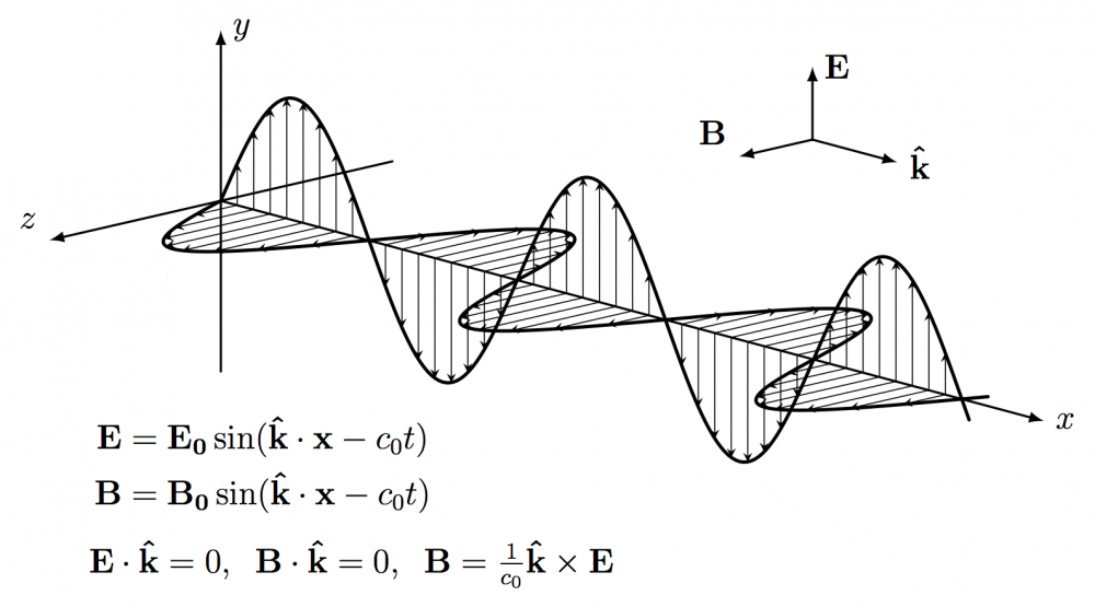
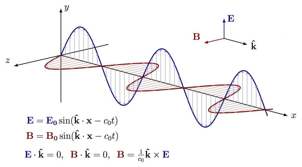
              \begin              {                              tikzpicture                }[                ten=(-15:i.ii), y=(xc:i.0), z=(-150:1.0),                     line cap=round, line bring together=round,                     axis/.style={black, thick,->},                     vector/.style={>=stealth,->}                ]                \large                \                def                \A                {1.5}                \                def                \nNodes{five              }              % employ fifty-fifty number              \              def              \nVectorsPerNode              {              eight}                \                def                \N                {                \nNodes*40}                \                def                \xmax                {                \nNodes*pi/2*1.01}                \pgfmathsetmacro                \nVectors                {(\nVectorsPerNode+1)*\nNodes                }                \                def                \vE                {                \mathbf                {E}}                \                def                \vB                {                \mathbf                {B}}                \                def                \vk                {                \mathbf                {                \hat                {k}}}                \draw                [                very thick,variable=\t,domain=0:\nNodes*pi/2*one.01,samples=\N                                ]                plot (\t,{                \A*sin(\t*360/pi)},0);                \draw                [                very thick,variable=\t,domain=0:\nNodes*pi/2*ane.01,samples=\Due north                                ]                plot (\t,0,{                \A*sin(\t*360/pi)              });              % chief axes              \draw              [              axis              ]              (0,0,0) -- ++(\xmax*1.1,0,0) node[              correct              ]              {                              $x$                };                \draw                [                centrality                ]                (0,-\A*1.4,0) -- (0,\A*1.four,0) node[                right                ]                {                $y$                };                \draw                [                axis                ]                (0,0,-\A*i.4) -- (0,0,\A*one.iv) node[                above left                ]                {                $z$                            };              % ...              \terminate              {                              tikzpicture                            }            

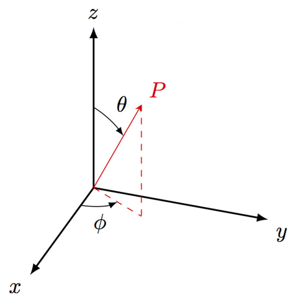
3D axis with spherical coordinates & CMS coordinate system

This piece of lawmaking is based on this StackExchange thread. It is a simple do in making axes and labeling angles in 3D. \usepackage{tikz-3dplot} needs to exist included. The full code can be found here.

                \tdplotsetmaincoords                {                sixty}{110}                  \begin                  {                  tikzpicture                                }[                calibration=3,tdplot_main_coords                ]                % variables                \                def                \rvec                {                .8}                  \                  def                  \thetavec                  {30}                  \                  def                  \phivec{sixty                }                % axes & vector                \coordinate                (O) at (0,0,0);                \draw                [                thick,->                ]                (0,0,0) -- (1,0,0) node[                ballast=north e                ]{                                  $x$                  };                  \depict                  [                  thick,->                  ]                  (0,0,0) -- (0,1,0) node[                  anchor=north west                  ]{                  $y$                  };                  \draw                  [                  thick,->                  ]                  (0,0,0) -- (0,0,ane) node[                  anchor=southward                  ]{                  $z$                  };                  \tdplotsetcoord                  {P}{                  \rvec                  }{                  \thetavec                  }{                  \phivec                  }                  \draw                  [                  -stealth,color=cherry                  ]                  (O) -- (P) node[                  to a higher place correct                  ]                  {                  $P$                                };                % arcs                \describe                [                dashed, color=red                ]                (O) -- (Pxy);                \describe                [                dashed, color=blood-red                ]                (P) -- (Pxy);                \tdplotdrawarc                [                ->                ]{                (O)}{0.2}{0}{\phivec                  }                  {anchor=north}{                  $\phi$                  }                  \tdplotsetthetaplanecoords                  {                  \phivec                  }                  \tdplotdrawarc                  [                  ->,tdplot_rotated_coords                  ]{(0,0,0)}{0.5}{0}{                  \thetavec                  }                  {anchor=south west}{                  $\theta$                  }                  \end                  {                  tikzpicture                                }              

An example of rotating the 3D axes with the CMS conventional coordinate system past using the option rotate around x=<angle> and more than (total lawmaking):

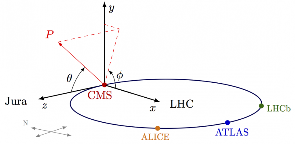
              % CMS conventional coordinate system with LHC and other detectors              \tdplotsetmaincoords              {              75}{50              }              % to reset previous setting              \begin              {                              tikzpicture                            }[              scale=two.seven,tdplot_main_coords,rotate effectually 10=90              ]              % variables              \              def              \rvec              {              1.two}                \                def                \thetavec                {40}                \                def                \phivec                {70}                \                def                \R                {one.1}                \                def                \w{0.three              }              % axes              \coordinate              (O) at (0,0,0);              \describe              [              thick,->              ]              (0,0,0) -- (i,0,0) node[              beneath left              ]{                              $x$                };                \draw                [                thick,->                ]                (0,0,0) -- (0,1,0) node[                below right                ]{                $y$                };                \draw                [                thick,->                ]                (0,0,0) -- (0,0,1) node[                below right                ]{                $z$                };                \tdplotsetcoord                {P}{                \rvec                }{                \thetavec                }{                \phivec                            }              % vectors              \draw              [              ->,red              ]              (O) -- (P) node[              above left              ]              {                              $P$                            };              \draw              [              dashed,red              ]              (O)  -- (Pxy);              \draw              [              dashed,cerise              ]              (P)  -- (Pxy);              \draw              [              dashed,scarlet              ]              (Py) -- (Pxy);              % circumvolve - LHC              \tdplotdrawarc              [              thick,rotate around ten=90,blackness!lxx!blue              ]{              (\R,0,0)}{                \R}{0}{360}{}{              }              % compass - the line betwixt CMS and ATLAS has a ~12° declination (http://googlecompass.com)              \brainstorm              {                              scope                }[                shift={(1.1*\R,0,1.65*\R)},rotate around y=12                ]                \describe                [                <->,blackness!50                ]                (-\w,0,0) -- (\w,0,0);                \draw                [                <->,black!l                ]                (0,0,-\w) -- (0,0,\w);                \node                [                above left,blackness!50,scale=0.6                ]                at (-\due west,0,0)                {Due north};                \end                {                telescopic                            }              % nodes              \node              [              left,marshal=center              ]              at (0,0,1.1)              {              Jura};                \node                [                correct                ]                at (\R,0,0)                {LHC};                \fill up                [                radius=0.8pt,black!20!cerise                ]                (O) circle node[                left=4pt,below=2pt] {CMS              };              \depict              [              thick              ]              (0.02,0,0) -- (0.v,0,0);              % partially overdraw x-axis and CMS indicate              \fill              [              radius=0.8pt,black!20!blueish              ]              (2*\R,0,0) circle     node[              correct=4pt,below=2pt,calibration=0.9              ]              {              ATLAS};                \make full                [                radius=0.8pt,black!10!orange                ]                ({                \R*sqrt(two)/2+\R                },0,{                \R*sqrt(2)/two              }) circle              % 45 degrees from ATLAS              node[              left=2pt,beneath=2pt,scale=0.8              ]              {              ALICE};                \fill                [                radius=0.8pt,black!60!green                ]                ({                \R*sqrt(2)/2+\R                },0,{-\R*sqrt(two)/2              }) circle              % 45 degrees from ATLAS              node[              beneath=2pt,right=2pt,scale=0.8              ]              {              LHCb              };              % arcs              \tdplotdrawarc              [              ->              ]{              (O)}{0.2}{0}{\phivec                }                {above=2pt,right=-1pt,anchor=mid west}{                $\phi$                }                \tdplotdrawarc                [                ->,rotate around z=\phivec-90,rotate around y=-ninety                ]{(0,0,0)}{0.five}{0}{                \thetavec                }                {anchor=mid eastward}{                $\theta$                }                \end                {                tikzpicture                            }            

Tau lepton decay signatures

Physics exercise

Higgs disuse planes

Bear on parameters

Examples of defining impact parameters in proton collisions (full lawmaking).

Timelines and scales

Examples of a uncomplicated time or energy scale with labels and arrows (full code).

Random timeline:

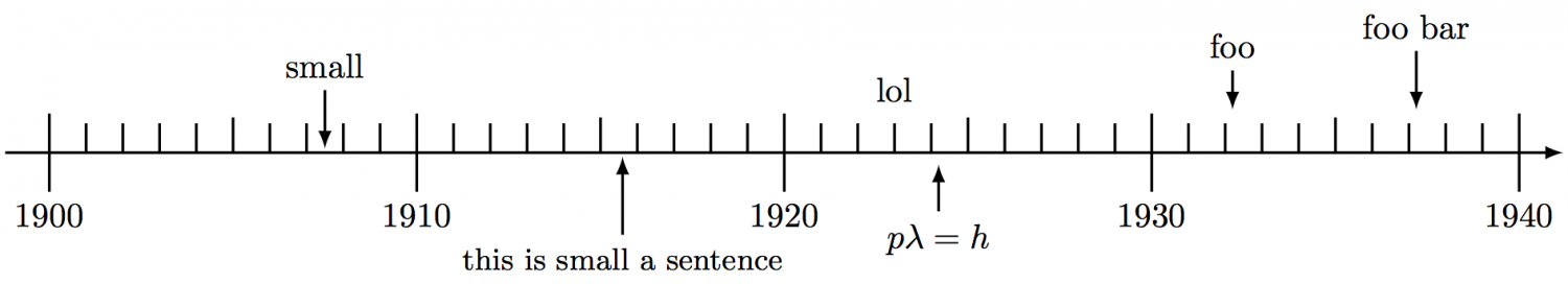
Logarithmic free energy scale of particle physics:

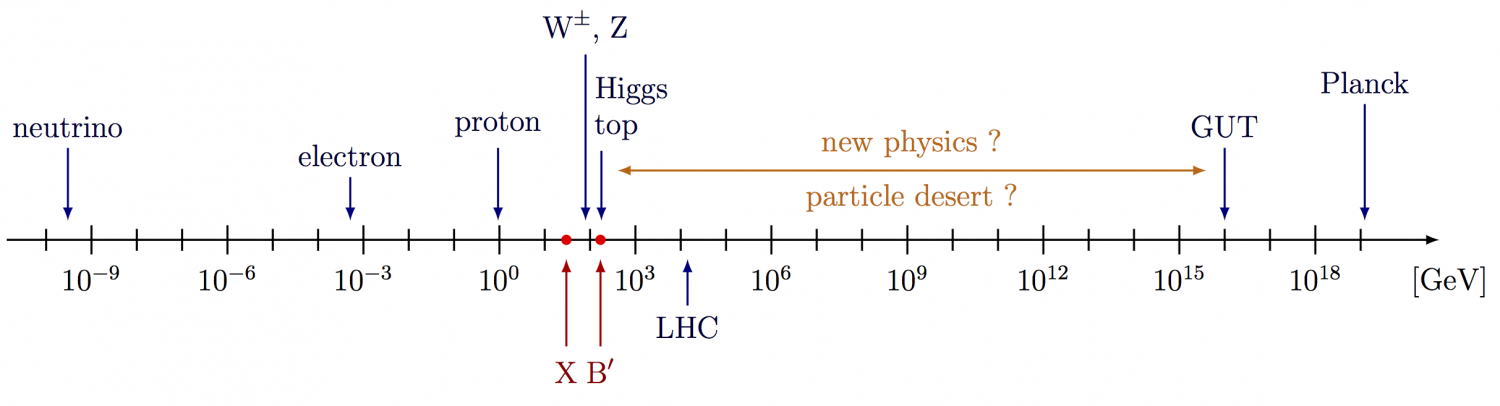
Timeline of particle physics (inspiration):
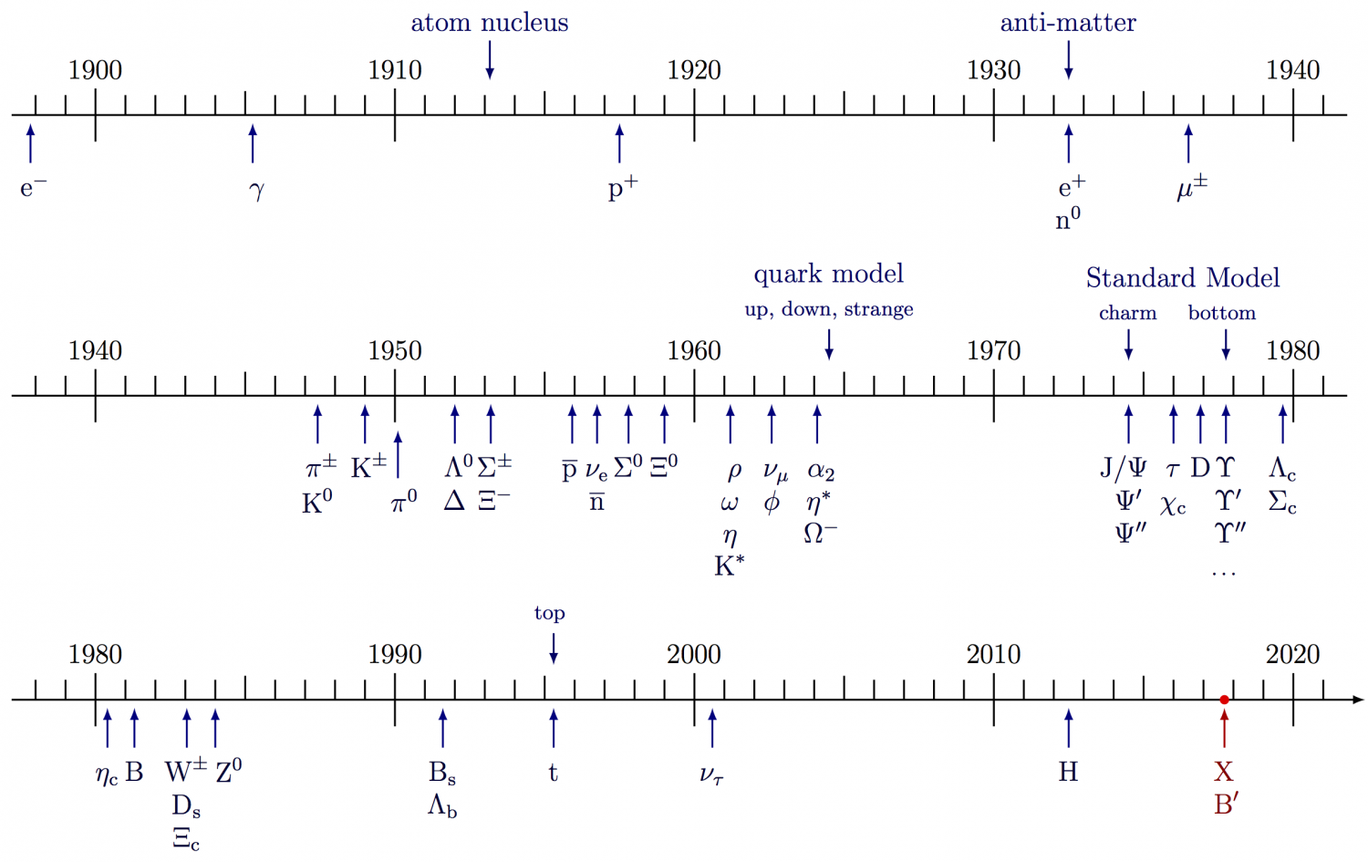
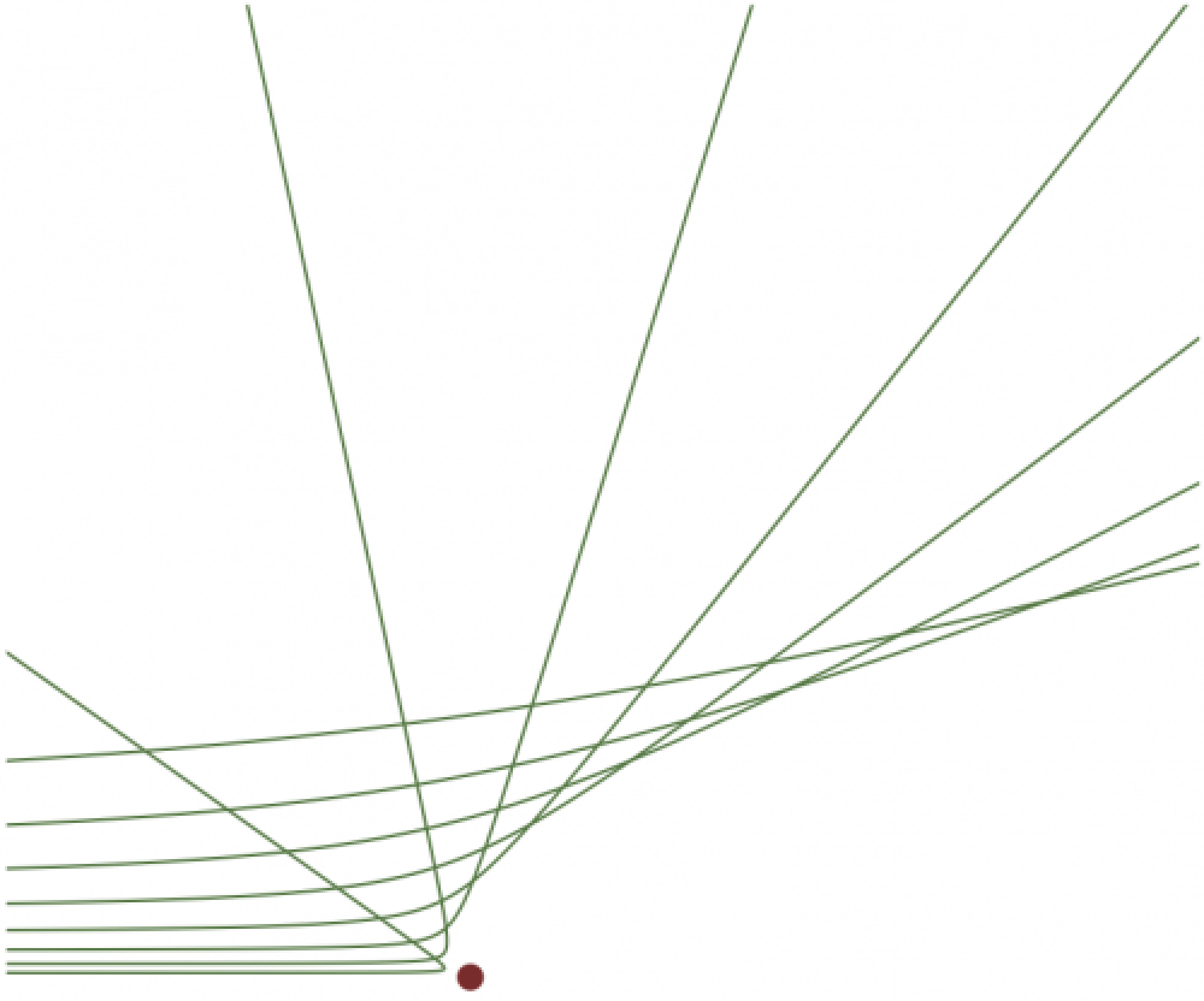
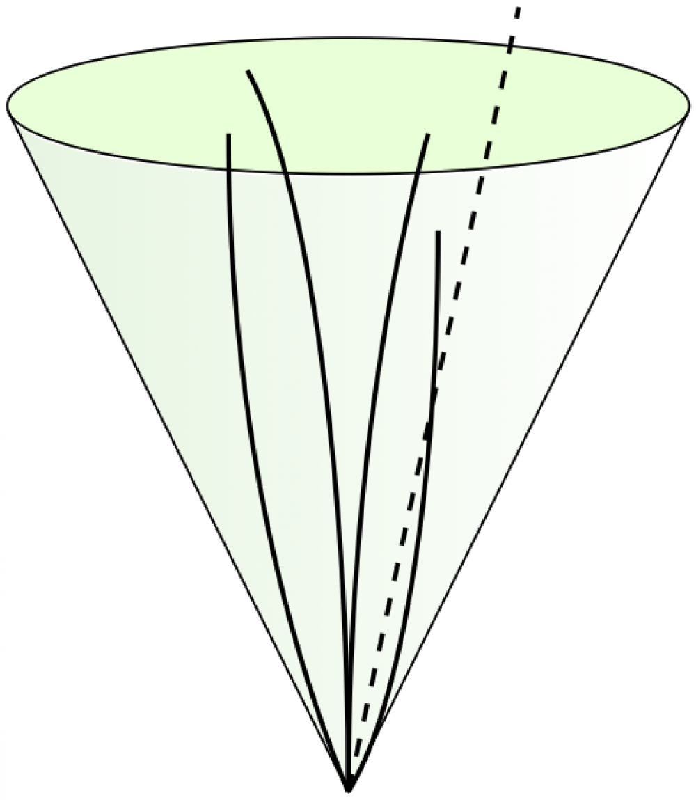
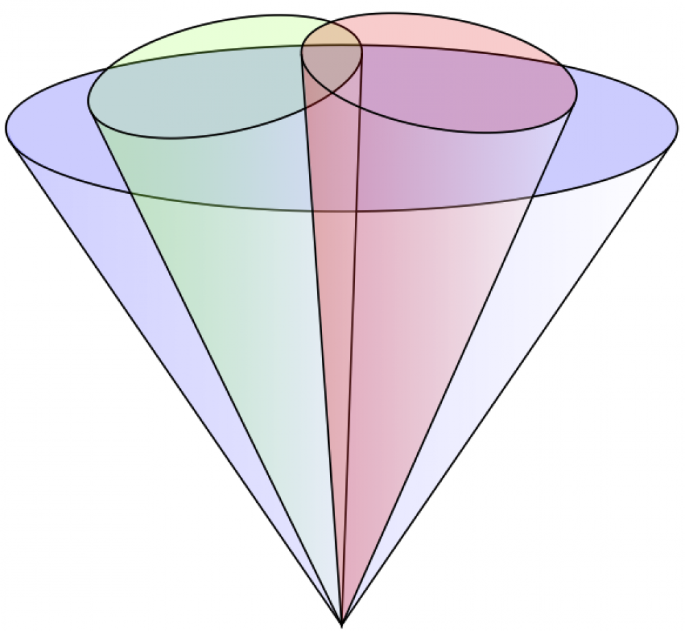
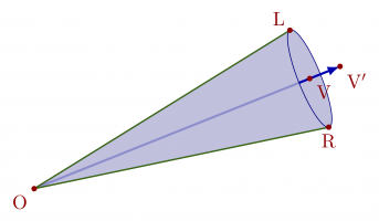
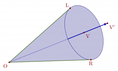
Jets cones

2 examples of cones. Full code tin can exist establish here.

                \begin                {                                  tikzpicture                                }                % cone variables                \                def                \x                {                ii.0}                  \                  def                  \y                  {four.0}                  \                  def                  \R                  {                  \x                  }                  \                  def                  \yc                  {                  \y+0.02}                  \                  def                  \due east{0.4                }                % cone shades + frame                \shade                [                right colour=white,left color=mylightgreen,opacity=0.iii                ]                (-\x,\yc) -- (-2,4) arc (180:360:{                                  \R                  }                  and                  \e) -- (\x,\yc) -- (0,0) -- bicycle;                  \describe                  [                  make full=green,opacity=0.two                  ]                  (0,\yc) circle ({                  \R                  }                  and                  \e);                  \depict                  (-\x,\y) -- (0,0) -- (\x,\y);                  \draw                  (0,\yc) circle ({                  \R                                }                and                \e);                % tracks                \draw                [                thick                ]                (0,0) arc (320:360:-three and 6.0);                %node[above] {1};                \depict                [                thick                ]                (0,0) arc (-70:  0:0.eight and 3.v);                %node[in a higher place] {2};                \draw                [                thick                ]                (0,0) arc (  0: lxx:0.nine and 4.5);                %node[above] {iii};                \depict                [                thick                ]                (0,0) arc (180:140:two and six.0);                %node[in a higher place] {4};                \draw                [                thick,dashed                ]                (0,0) -- (1,4.6);                \finish                {                                  tikzpicture                                }              

                \begin                {                                  tikzpicture                                }                % AK8 variables                \                def                \ten                {                2.4}                  \                  def                  \y                  {3.v}                  \                  def                  \R                  {                  \ten+0.02}                  \                  def                  \yc                  {                  \y+0.08}                  \                  def                  \e{0.6                }                % AK8 cone                \shade                [                right color=white,left color=bluish,opacity=0.two                ]                (-\x,\y) -- (-\ten,\yc) arc (180:360:{                                  \R                  }                  and                  \e) -- (\ten,\y) -- (0,0) -- bicycle;                  \draw                  [                  fill=blue,opacity=0.2                  ]                  (0,\yc) circumvolve ({                  \R                  }                  and                  \east);                  \describe                  (-\ten,\y) -- (0,0) -- (\x,\y);                  \draw                  (0,\yc) circle ({                  \R                                }                and                \due east);                % AK4 variables                \                def                \ten                {                i.0}                  \                  def                  \y                  {4.0}                  \                  def                  \R                  {                  \x+0.005}                  \                  def                  \yc                  {                  \y+0.04}                  \                  def                  \east{0.iv                }                % AK4 cone 1                \begin                {                                  scope                  }[                  rotate=12                  ]                  \shade                  [                  correct color=white,left color=greenish,opacity=0.iii                  ]                  (-\x,\yc) -- (-\10,\yc) arc (180:360:{                  \R                  }                  and                  \e) -- (\ten,\yc) -- (0,0) -- cycle;                  \describe                  [                  fill=green,opacity=0.two                  ]                  (0,\yc) circle ({                  \R                  }                  and                  \east);                  \draw                  (-\x,\y) -- (0,0) -- (\x,\y);                  \describe                  (0,\yc) circle ({                  \R                  }                  and                  \due east);                  \finish                  {                  scope                                }                % AK4 cone ii                \begin                {                                  scope                  }[                  rotate=-x                  ]                  \shade                  [                  right color=white,left colour=red,opacity=0.iii                  ]                  (-\x,\yc) -- (-\x,\yc) arc (180:360:{                  \R                  }                  and                  \due east) -- (\x,\yc) -- (0,0) -- cycle;                  \describe                  [                  fill=ruby-red,opacity=0.2                  ]                  (0,\yc) circle ({                  \R                  }                  and                  \e);                  \draw                  (-\x,\y) -- (0,0) -- (\x,\y);                  \depict                  (0,\yc) circle ({                  \R                  }                  and                  \due east);                  \finish                  {                  scope                  }                  \end                  {                  tikzpicture                                }              

Tiptop jets

The full code can be found here.

            \            newcommand            \jetcone            [            5            ][            blueish            ]{                          {              \pgfmathanglebetweenpoints              {              \pgfpointanchor              {#2}{center}}{              \pgfpointanchor              {#3}{middle}}              \              edef              \ang              {#4/2}              \              edef              \east              {#five}              \              edef              \vang              {              \pgfmathresult                        }            % angle of vector OV            \tikzmath            {            coordinate            \C;            \C            = (#2)-(#iii);            \x            = veclen(\Cx,\Cy)*\e*sin(\ang)^2;            % 10 coordinate P            \y            = tan(\ang)*(veclen(\Cx,\Cy)-\x);            % y coordinate P            \a            = veclen(\Cx,\Cy)*sqrt(\east)*sin(\ang);            % vertical radius            \b            = veclen(\Cx,\Cy)*tan(\ang)*sqrt(1-\e*sin(\ang)^2);            % horizontal radius            \angb            = acos(sqrt(\eastward)*sin(\ang));            % bending of P in ellipse            }            \coordinate            (tmpL) at ($(#3)-(\vang:\ten              pt)+(\vang+90:\y              pt)$);            % tangency            \draw            [            thin,#i!40!black,fill=#1!50!black!80,rotate=\vang                        ]            (#iii) ellipse({                          \a              pt}              and              {              \b              pt});              \draw              [              sparse,#ane!40!black,fill=#1!80!black!40,rotate=\vang                            ]              (tmpL) arc(180-\angb:180+\angb:{              \a              pt}              and              {              \b              pt})     -- ($(#2)+(\vang:0.018)$) -- bike;              }}              \brainstorm              {              tikzpicture              }              \              def              \R{2.5            }            \coordinate            (O) at (0,0);            \coordinate            (BJ) at ( 65:1.i*\R);            % b jet 1            \coordinate            (J1) at ( xv:ane.0*\R);            % q jet 1            \coordinate            (J2) at (-xx:1.0*\R);            % q jet two            \jetcone            [            green!80!black            ]{            O}{BJ}{14}{0.10}              \jetcone              {O}{J1}{16}{0.08}              \jetcone              {O}{J2}{16}{0.10}              \node              [              green!fifty!blackness              ]              at (65:i.24*\R)              {b};              \node              [              blue!80!black,correct              ]              at (-five:one.00*\R)              {              $\mathrm                {W}                \to                qq$              };              \end              {              tikzpicture                        }          

Jets vectors

One tin do some projections of jet and MET vectors to construct variables like MT2 in SUSY searches. The full code can be plant here.

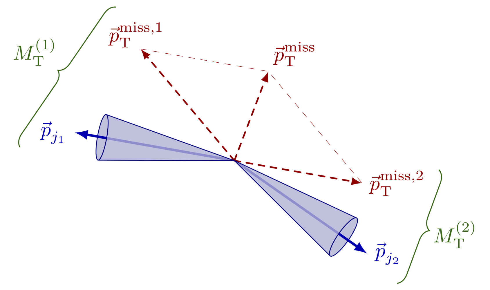
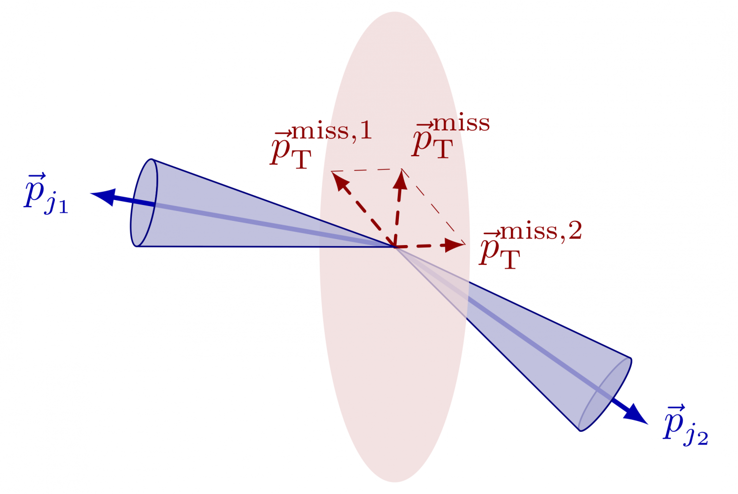
            \            newcommand            \jetcone            [            four            ]{                          \pgfmathanglebetweenpoints              {              \pgfpointanchor              {#1}{center}}{              \pgfpointanchor              {#ii}{center}}              \              edef              \tmpang              {              \pgfmathresult              }              \coordinate              (tmpC) at ($(#2)+(\tmpang-180:{abs(#four)+0.4})$);            % center            \coordinate            (tmpL) at ($(tmpC)+(\tmpang+90:#3)$);            % left corner            \coordinate            (tmpR) at ($(tmpC)+(\tmpang-90:#three)$);            % right corner            \draw            [            cone,rotate=\tmpang                        ]            %(tmpR) arc(ninety:-90:{#4} and {#3});            (tmpC) ellipse({            #4}              and              {#3});              \begin              {              telescopic              }              \clip              [              rotate=\tmpang                            ]              (tmpR) -- (#1) -- (tmpL) arc(ninety:-ninety:{#four+0.six}              and              {#3});              \draw              [              vector              ]              (#ane) -- (#2);              \end              {              scope              }              \describe              [              cone,rotate=\tmpang                            ]              (tmpL) arc(90:270:{#4}              and              {#3}) -- (#one) -- cycle;                        }            % MT2            \begin            {                          tikzpicture              }              \              def              \R{two.8            }            \coordinate            (O) at (0,0);            \coordinate            (J1) at (170:\R);            % jet 1 pT            \coordinate            (J2) at (-35:\R);            % jet 2 pT            \coordinate            (M1) at (130:0.ix*\R);            % pTmiss component 1            \coordinate            (M2) at (-10:0.8*\R);            % pTmiss component two            \coordinate            (One thousand) at ($(M1)+(M2)$);            % total missing momentum            % PTMISS            \draw            [            ptmiss,-,very thin            ]            (M1) -- (Thousand) -- (M2);            \describe            [            ptmiss            ]            (O) -- (M1) node[            left=ii,in a higher place=-3            ]            {                          $\ptmissX{ane}$              };              \draw              [              ptmiss              ]              (O) -- (M2) node[              correct=0              ]              {              $\ptmissX{two}$              };              \draw              [              ptmiss              ]              (O) -- (1000) node[              to a higher place right=-1              ]              {              $\ptmiss$                        };            % JET CONES            %\draw[vector] (O) -- (J1);            %\draw[vector] (O) -- (J2);            %\cone{O}{J1}{0.3}{0.15}            \jetcone            {            O}{J1}{0.iv}{0.08}              \jetcone              {O}{J2}{0.4}{0.10}              \node              [              vector,left              ]              at (J1)              {              $\vv{p}_{j_1}$              };              \node              [              vector,right              ]              at (J2)              {              $\vv{p}_{j_2}$                        };            % CURLY Brace            \draw            [            line width=0.5,mygreen,decorate,ornament={brace,aamplitude=six}              ]              ($(J1)+(195:0.35*\R)$) -- ($(M1)+(120:0.30*\R)$) node[              midway,above left=2              ]              {              $\MTX{ane}$              };              \draw              [              line width=0.5,mygreen,decorate,decoration={brace,amplitude=half-dozen}              ]              ($(M2)+(10:0.48*\R)$) -- ($(J2)+(-45:0.26*\R)$) node[              midway,below=four,correct=4              ]              {              $\MTX{2}$              };              \end              {              tikzpicture                        }          

Tangent to a circle or ellipse

Some dissimilar methods of finding the tangent to a circumvolve or ellipse in TikZ. Using these methods a nice cone can be fabricated. The total code can exist institute here.

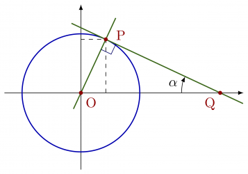
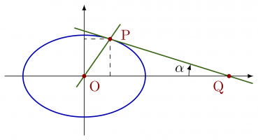
            % TANGENT to CIRCLE - known: r, q            \begin            {                          tikzpicture              }              \              def              \r{1.5            }            % radius            \            def            \q            {            4            }            % altitude center-external point q = |OQ|            \            def            \x            {            {\r^2/\q}            }            % Q x coordinate            \            def            \y            {            {\r*sqrt(ane-(\r/\q)^2}            }            % Q y coordinate            \coordinate            (O) at (0,0);            % circle center O            \coordinate            (Q) at (\q,0);            % external point Q            \coordinate            (P) at (\10,\y);            % point of tangency, P            \describe            [            ->            ]            (0,-1.iii*\r) -- (0,1.5*\r);            \draw            [            ->            ]            (-one.3*\r,0) -- (\q+0.four*\r,0);            \draw            [            dashed            ]            (\x,0) |- (0,\y);            \draw            [            myblue,thick            ]            (O) circle(\r);            \describe            [            mygreen,thick            ]            ($(Q)!-0.2!(P)$) -- ($(Q)!1.three!(P)$);            \depict            [            mygreen,thick            ]            ($(O)!-0.3!(P)$) -- ($(O)!one.4!(P)$);            \rightAngle            {            Q}{P}{O}{0.forty}              \make full              [              myred              ]              (O) circle(0.05) node[              below right              ]              {O};              \make full              [              myred              ]              (Q) circumvolve(0.05) node[              below left              ]              {Q};              \fill up              [              myred              ]              (P) circle(0.05) node[              above=3,correct=iv              ]              {P};              \finish              {              tikzpicture                        }            % TANGENT to ELLIPSE - known: a, b, q            \begin            {                          tikzpicture              }              \              def              \a{1.five            }            % horizontal radius            \            def            \b            {            i.0            }            % vertical radius            \            def            \q            {            4            }            % distance middle-external point q = |OQ|            \            def            \x            {            {\a^2/\q}            }            % ten coordinate P            \            def            \y            {            {\b*sqrt(one-(\a/\q)^2}            }            % y coordinate P            \coordinate            (O) at (0,0);            % circle center O            \coordinate            (Q) at (\q,0);            % external point Q            \coordinate            (P) at (\x,\y);            % point of tangency, P            \draw            [            ->            ]            (0,-\b-0.3*\a) -- (0,\b+0.4*\a);            \depict            [            ->            ]            (-one.3*\a,0) -- (\q+0.four*\a,0);            \describe            [            dashed            ]            (\x,0) |- (0,\y);            \draw            [            myblue,thick            ]            (O) ellipse({                          \a              }              and              {              \b              });              \draw              [              mygreen,thick              ]              ($(Q)!-0.2!(P)$) -- ($(Q)!1.3!(P)$);              \draw              [              mygreen,thick              ]              ($(O)!-0.3!(P)$) -- ($(O)!1.4!(P)$);              \fill              [              myred              ]              (O) circle(0.05) node[              below right              ]              {O};              \fill up              [              myred              ]              (Q) circumvolve(0.05) node[              below left              ]              {Q};              \make full              [              myred              ]              (P) circle(0.05) node[              above=three,right=4              ]              {P};              \end              {              tikzpicture                        }          

Source: https://wiki.physik.uzh.ch/cms/latex:tikz

Posted by: doranspold1936.blogspot.com

0 Response to "How To Draw A Figure In Latex"

Post a Comment

Iklan Atas Artikel

Iklan Tengah Artikel 1

Iklan Tengah Artikel 2

Iklan Bawah Artikel